Joining relations

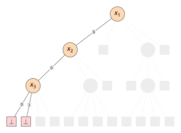
Joining like a DB Dude

$Q \coloneq R(x_1, x_2) \wedge S(x_1, x_3) \wedge T(x_2, x_3)$

$R$	$x_1$	$x_2$
	0	0
	0	1
	2	1

$S$	$x_1$	$x_3$
	0	0
	0	2
	2	3

$T$	$x_2$	$x_3$
	0	2
	1	0
	1	2

Devise a query plan: $(R \bowtie S)$ $\bowtie T$
Materialize the intermediate joins.

$x_1$	$x_2$	$x_3$
0	0	0
0	0	2
0	1	0
0	1	2
2	1	3

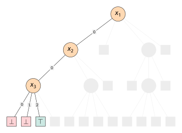
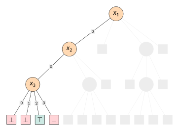
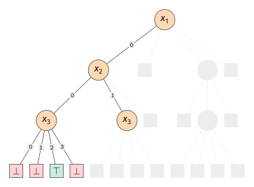
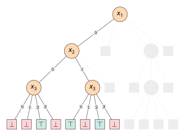
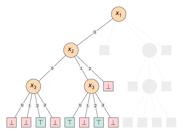
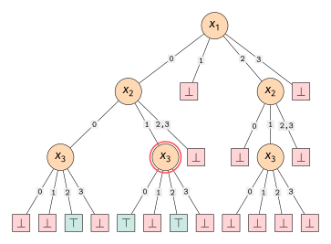
Joining like a SAT Guy

$Q \coloneq R(x_1, x_2) \wedge S(x_1, x_3) \wedge T(x_2, x_3)$

$R$	$x_1$	$x_2$
	0	0
	0	1
	2	1

$S$	$x_1$	$x_3$
	0	0
	0	2
	2	3

$T$	$x_2$	$x_3$
	0	2
	1	0
	1	2

Disruptive poll

In theory, is it better to do a database join like:

A DB Dude
A SAT guy

No confidence vote

Go home, you are not qualified to talk about joins after saying dumb things like that.
This is LE CRIL. We do SAT before breakfast everyday. Some of us even replace sugar with GLUCOSE in their coffee. Tell us the whole story

What is wrong with joining like a pro

$Q \coloneq R(x_1, x_2) \wedge S(x_1, x_3) \wedge T(x_2, x_3)$

It is known that if $|R^\mathbb{D}|, |S^\mathbb{D}|, |T^\mathbb{D}| \leq N$ , then $|Q(\mathbb{D})| \leq N^{1.5}$ .
$R \bowtie S$ may have $N^2$ answers!

Worst scenario for query plans

Consider $\mathbb{D}$ on domain $D = D_1 \uplus D_2 \uplus D_3$ with:

$0 \notin D$
$|D_1|=|D_2|=|D_3|=N$ .

$R$	$x_1$	$x_2$
	0	$D_2$
	$D_1$	0

$S$	$x_1$	$x_3$
	0	$D_3$
	$D_1$	0

$T$	$x_2$	$x_3$
	0	$D_3$
	$D_2$	0

$|R^\mathbb{D}\bowtie S^\mathbb{D}| \geq N^2$ , $|R^\mathbb{D}\bowtie T^\mathbb{D}| \geq N^2$ , $|S^\mathbb{D}\bowtie T^\mathbb{D}| \geq N^2$
$|Q(\mathbb{D})| = 0$ .

Every query plan will materialize a table of size $O(N^2)$ but the answer table will never be of size greater than $(2N)^{1.5}$ .

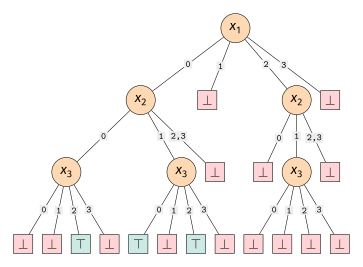
And the brute?

Domain $D = D_1 \uplus D_2 \uplus D_3$ with $0 \notin D$ and $|D_1|=|D_2|=|D_3|=N$ .

$R$	$x_1$	$x_2$
	0	$D_2$
	$D_1$	0

$S$	$x_1$	$x_3$
	0	$D_3$
	$D_1$	0

$T$	$x_2$	$x_3$
	0	$D_3$
	$D_2$	0

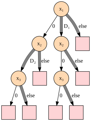
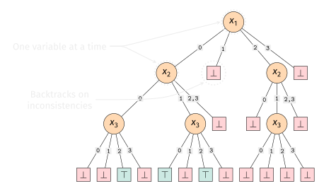
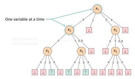
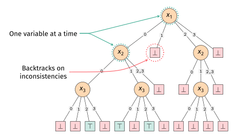
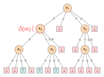
If we do the “else” branches efficiently (e.g. by reading values from one table), the algorithm makes $O(N)$ recursive calls.

Worst-case optimality

Worst-case optimal join

$Q \coloneq R(x_1, x_2) \wedge S(x_1, x_3) \wedge T(x_2, x_3)$

Ideal complexity: output $Q(\mathbb{D})$ in time $O(f(|Q|) \cdot |Q(\mathbb{D})|)$ …

… unlikely to be possible.

Worst case optimal: output $Q(\mathbb{D})$ in time $\tilde{O}(f(|Q|) \cdot N^{1.5})$ .

$N$ is the size of the largest input relation and $\tilde{O}(\cdot)$ ignores polylog factors.

$f(|Q|)$ : data complexity, ie, $Q$ is considered constant. Ideally, $f$ is a reasonable polynomial though.

Worst case value

Consider a join query $Q$ and all databases for $Q$ with a bound $N$ on the table size: $\mathcal{D}_{Q}^{\leqslant N}= \{\mathbb{D}\mid \forall R \in Q, |R^\mathbb{D}| \leqslant N\}$ and let: $\mathsf{wc}(Q, N) = \mathsf{sup}_{\mathbb{D}\in\mathcal{D}_{Q}^{\leqslant N}}~|Q(\mathbb{D})|$

$\mathsf{wc}(Q,N)$ is the worst case: the size of the biggest answer set possible with query $Q$ and databases where each table are bounded by $N$ .

Worst case examples

Cartesian product: $Q_2 = R_1(x_1) \wedge R_2(x_2)$ has $\mathsf{wc}(Q_2,N) = N^2$ .
Similarly: $Q_k = R_1(x_1) \wedge \dots \wedge R_k(x_k)$ has $\mathsf{wc}(Q_2,N) = N^k$ .
Square query: $Q_\square = R(x_1,x_2) \wedge R(x_2,x_3) \wedge R(x_3,x_4) \wedge R(x_4,x_1)$ has $\mathsf{wc}(Q_\square,N)=N^2$ .
Triangle query: $Q_\Delta = R(x, y) \wedge S(x, z) \wedge T(y, z)$ , $\mathsf{wc}(Q_\Delta, N) = N^{1.5}$ .
The n-cycle: $Q_{C_n}(x_1,\dots,x_n) = R_1(x_1,x_2) \wedge R_2(x_2,x_3) \wedge \dots \wedge R_n(x_{n},x_1)$ : $\mathsf{wc}(Q_{C_n})=N^\frac{n}{2}$ .

We know how to compute $\rho(Q)$ such that $\mathsf{wc}(Q,N) = \tilde{O}(N^{\rho(Q)})$ but we do not need it!

This is known as the AGM-bound

Worst case optimal join (WCOJ) algorithms

A join algorithm is worst case optimal (wrt $\mathcal{D}_{Q}^{\leqslant N}$ ) if for every $Q$ , $N \in \mathbb{N}$ and $\mathbb{D}\in \mathcal{D}_{Q}^{\leqslant N}$ , it computes $Q(\mathbb{D})$ in time $\tilde{O}(f(|Q|) \cdot \mathsf{wc}(Q,N))$

Data complexity model: $Q$ considered constant hence $f(|Q|)$ also.
In this talk, $f$ will be a reasonable polynomial!

The DBMS approach is not worst case optimal (triangle example from before).

Existing WCOJ Algorithm

Rich literature:

NPRR join (Ngo, Porat, Ré, Rudra, PODS12): usual join plans but with relations partitionned into high/low degree tuples.
Leapfrog Triejoin (Veldhuizen, ICDT14)
Generic Join (Ngo, PODS18): both branch and bound algorithms as ours but more complex analysis/data structures.
PANDA (PODS17): handle complex database constraints, very complex, long analysis.

We prove the worst case optimality of the branch and bound algorithm in an elementary way.

Analysing the brute

Algorithm reminder

Complexity analysis

One recursive call:

branch variable $x_i$ on value $d \in \mathsf{dom}$
filter/project relations with $x_i$
Binary search in $O(\log |R|)$ if $R$ ordered
( $O(1)$ possible using tries).

$R$	$x_1$	$x_2$
▸	0	0
	0	2
▸	1	0
	1	1	◂
	2	0
	2	1	◂

Total complexity: number of recursive calls times $\tilde{O}(m)$ where $m$ is the number of atoms.

Number of calls: example

Nodes: partial assignment $\tau$
Here: $\tau := \{x_1=0, x_2=1\}$
Not node: partial assignment compatible with every relation
$\tau$ solution of $Q_2(\mathbb{D}_2)$ : project on $x_1,x_2$ .
At most: $|Q_2(\mathbb{D}_2)|$ such nodes at level $3$

$Q \coloneq R(x_1, x_2) \wedge S(x_1, x_3) \wedge T(x_2, x_3)$

$R$	$x_1$	$x_2$
	0	0
	0	1
	2	1

$S$	$x_1$	$x_3$
	0	0
	0	2
	2	3

$T$	$x_2$	$x_3$
	0	2
	1	0
	1	2

$Q_2 \coloneq R_2(x_1, x_2) \wedge S_2(x_1) \wedge T_2(x_2)$

$R_2$	$x_1$	$x_2$
	0	0
	0	1
	2	1

$S_2$	$x_1$
	0
	2

$T_2$	$x_2$
	0
	1

Number of calls in general

a call = a node = a partial assignment.
τ:=x1=d1,…,xi=di\tau := x_1=d_1, \dots, x_i=d_i current call, not :
- No inconsistency.
- $R^\mathbb{D}[\tau]$ not empty for each $R \in Q$
- $\tau \in Q_i(\mathbb{D})$ for $Q_i = \bigwedge_{R\in Q}\prod_{x_1\dots x_i} R$
- $\leq \sum_{i=1}^n |Q_i(\mathbb{D})|$ such nodes!

τ:=x1=d1,…,xi+1=di+1\tau := x_1=d_1, \dots, x_{i+1}=d_{i+1} current call is :
- $x_1=d_1, \dots, x_{i}=d_i$ is not $\bot$ .
- $\leq |\mathsf{dom}| \cdot \sum_{i=1}^n |Q_i(\mathbb{D})|$ $\bot$ -nodes!

At most $(|\mathsf{dom}|+1) \sum_{i=1}^n |Q_i(\mathbb{D})|$ calls.

Complexity: $\tilde{O}(m|\mathsf{dom}|\cdot \sum_{i=1}^{n}|Q_i(\mathbb{D})|)$ .

Toward worst case optimality

$\begin{align*} |Q_i(\mathbb{D})| &= |\bigwedge_{R\in Q}\prod_{x_1\dots x_i} R^\mathbb{D}|\\ &= |\bigwedge_{R\in Q} R^{\mathbb{D}'}| \\ &= |Q(\mathbb{D}')| \end{align*}$

where $R^{\mathbb{D}'} = \prod_{x_1\dots x_i} R^\mathbb{D}\times \{0\}^{X_R \setminus x_1, \dots, x_i}$

Crucial observation:

$|R^{\mathbb{D}'}| = |\prod_{x_1\dots x_i} R^\mathbb{D}| \leq |R^\mathbb{D}| \leq N$
Hence $\mathbb{D}' \in \mathcal{D}_{Q}^{\leqslant N}$ .
$|Q_i(\mathbb{D})| = |Q(\mathbb{D}')| \leq \mathsf{wc}(Q,N)$

$\mathbb{D}$

$R$	$x_1$	$x_2$
	0	0
	0	1
	2	1

$S$	$x_1$	$x_3$
	0	0
	0	2
	2	3

$T$	$x_2$	$x_3$
	0	2
	1	0
	1	2

$\mathbb{D}_2$

$R_2$	$x_1$	$x_2$
	0	0
	0	1
	2	1

$S_2$	$x_1$
	0
	2

$T_2$	$x_2$
	0
	1

$\mathbb{D}'$

$R'$	$x_1$	$x_2$
	0	0
	0	1
	2	1

$S'$	$x_1$	$x_3$
	0	0
	2	0

$T'$	$x_2$	$x_3$
	0	0
	1	0

Branch and bound complexity

$|Q_i(\mathbb{D})| \leq wc(Q,N)$

The complexity of the branch and bound algorithm is

$\tilde{O}(m|\mathsf{dom}|\cdot \sum_{i=1}^n|Q_i(\mathbb{D})|)$

$\tilde{O}(m|\mathsf{dom}| \cdot n\mathsf{wc}(Q, N))$

$\tilde{O}(mn \cdot |\mathsf{dom}| \cdot \mathsf{wc}(Q, N))$

$\tilde{O}(mn \cdot$ ${|\mathsf{dom}|}$ $\cdot \mathsf{wc}(Q, N))$

We do not even need to know $\mathsf{wc}(Q,N)$ to prove it!

Make the domain binary!

$R$	$x$	$y$
	1	2
	2	1
	3	0

⇝

$x^1$	$x^0$	$y^1$	$y^0$
0	1	1	0
1	0	0	1
1	1	0	0

$Q$ ⇝ $\tilde{Q}^b$ has $bn$ variables
$\mathbb{D}$ ⇝ $\tilde{\mathbb{D}}^b$ for $b = \log |\mathsf{dom}|$ . Database has roughly the same bitsize but size $2$ domain!

WCOJ finally

To compute Q(𝔻)Q(\mathbb{D}) run simple branch and bound algorithm on (Q̃b,𝔻̃b)(\tilde{Q}^b, \tilde{\mathbb{D}}^b):
- runs in time $\tilde{O}(m \cdot (n\log |\mathsf{dom}|) \cdot {\color{red}2} \mathsf{wc}(\tilde{Q}^{b}, N, 2))$
- where $\mathsf{wc}(\tilde{Q}^{b}, N, 2)$ is the worst case for $\tilde{Q}^b$ on relations of size $\leq N$ and domain $2$ .
- $\mathsf{wc}(\tilde{Q}^{b}, N, 2) \leq \mathsf{wc}(Q,N)$ by reconverting back to larger domain.

We hence compute $Q(\mathbb{D})$ in time $\tilde{O}(m n \cdot \mathsf{wc}(Q, N))$ !

Worst case and functional dependencies

Functional dependencies

$Q = R(x_1,x_2) \wedge S(x_2,x_3)$ .

We have: $\mathsf{wc}(Q,N) = N^2$ .

What if we know that every database verify a key constraint $x_2 \rightarrow x_1$ ?

(ie fixing the value of $x_2$ fixes the value of $x_1$ ).

The worst case is $N$ on such database!

Worst-case and constraints

$\mathsf{wc}(Q,N)$ :

Worst case for any database whose relation have size at most $N$ ,
ie every database respecting a cardinality constraint.

$\mathsf{wc}(Q,N,x\rightarrow y, z \rightarrow w \dots)$

Worst case for any database whose relation have size at most $N$ and respecting some “simple” functional dependencies.
May be smaller than $\mathsf{wc}(Q,N)$

$\mathsf{wc}(Q,\mathcal{C})$ :

More generally, worst case for a class $\mathcal{C}$ of databases.
More complex functional depencies $X \rightarrow y$ .
“Statistical” constraints (degree constraints)

Back to the example

$Q = R(x_1,x_2) \wedge S(x_2,x_3)$ .

We have:

$\mathsf{wc}(Q,N) = N^2$ .
$\mathsf{wc}(Q,N, x_2 \rightarrow x_1) = N$ .

Is our algorithm worst-case optimal for this class?

Yes if $x_2$ is set before $x_1$ : UNIT PROPAGATION!

More than one FD

$Q$ query
$\Sigma = \{x_1 \rightarrow y_1, x_2 \rightarrow y_2 \dots\}$ simple functional dependencies

$\Sigma$ is a directed graph: strong connected components induce a preorder $\prec$ on variables.

Branching Algorithm + Unit propagation following $\prec$ runs in time $\tilde{O}(|\mathsf{wc}(Q,N,\Sigma)|)$ !

“DPLL is worst-case optimal”!

Wrap up

Worst-case optimality is a cute concept!
Simple algorithm achieves it with a simple analysis
This is roughly DPLL (exhaustive) with static ordering.

How far can we push this and remain worst case optimal?

What about non simple functional dependencies?
“Statistical” constraints (as maintained by DBMS)
…

Les slides auxquelles vous avez échappé

Uniform Sampling of answers

Given $Q$ and $\mathbb{D}$ , sample $\tau \in Q(\mathbb{D})$ with probability $\frac{1}{|Q(\mathbb{D})|}$ or fail if $Q(\mathbb{D}) = \emptyset$ .

Naive algorithm by materialization: $\tilde{O}(\mathsf{wc}(Q,N) poly(|Q|))$ .

Algorithm by randomly navigating the tree: $\tilde{O}(\frac{\mathsf{wc}(Q,N)}{|Q(\mathbb{D})|+1} poly(|Q|))$ .

Degree Constraints

A degree constraint is a constraint $(X,Y,N_{Y|X})$ where $X \subseteq Y$ . A relation $R$ verifies the constraint if

$\max \{ |\prod_{Y} R[\tau]|, \tau \in \mathsf{dom}^X\} \leq N_{Y|X}$

Cardinality constraint = degree constraint with $X = \emptyset$ .
Functional dependency = degree constraint with $N_{Y|X} = 1$ .

Acyclic Degree Constraints

$\Delta = \{(X_1, Y_1, N_{1}) \dots, (X_k, Y_k, N_k)\}$ set of degree constraints.

$G(\Delta)$ : vertices are the variables and $x \rightarrow y$ if $x \in X_i$ and $y \in Y_i$ for some $i$ .
If $G(\Delta)$ is acyclic, then let $\pi = x_1,\dots,x_n$ be a topological sort of $G(\Delta)$ . Then

Our algorithm is worst case optimal wrt $\Delta$ (as long as we follow $\pi$ ).

"DPLL" is Worst Case Optimal

Joining relations

Joining like a DB Dude

Joining like a SAT Guy

Disruptive poll

No confidence vote

What is wrong with joining like a pro

Worst scenario for query plans

And the brute?

Worst-case optimality

Worst-case optimal join

Worst case value

Worst case examples

Worst case optimal join (WCOJ) algorithms

Existing WCOJ Algorithm

Analysing the brute

Algorithm reminder

Complexity analysis

Number of calls: example

Number of calls in general

Toward worst case optimality

Branch and bound complexity

Make the domain binary!

WCOJ finally

More on Binarization

Worst case and functional dependencies

Functional dependencies

Worst-case and constraints

Back to the example

More than one FD

Wrap up

Les slides auxquelles vous avez échappé

Uniform Sampling of answers

Degree Constraints

Acyclic Degree Constraints