Convex Hull of Boolean Functions

A picture is worth a thousand maybe two slides

$f$	$x$	$y$
$\vec{v}_0$	0	0
$\vec{v}_1$	1	0
$\vec{v}_2$	0	1

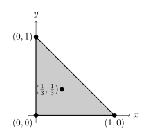
Convex Hull $conv(f)$ of $f$ : every convex combination of its models. Here :

$\lambda_0 \vec{v}_0 + \lambda_1 \vec{v}_1 + \lambda_2 \vec{v}_2$

with $\lambda_0+\lambda_1+\lambda_2=1$ are positive real numbers.

Eg $({1/3}, {1/3})$ is obtained as $(\vec{v}_0+\vec{v}_1+\vec{v}_2)/3$ .

Convex Hull and Polyhedron

$conv(f) \subseteq [0,1]^n$ is a bounded polyhedron.

$(x_1,\dots,x_n) = \sum_{\tau \models f} \lambda_\tau \vec\tau$

with $\sum_{\tau \models f} \lambda_\tau = 1$
$\lambda_\tau \geq 0$ .

Definition by linear constraints

$x_1 = \sum_{\tau \models f|_{x_1=1}} \lambda_\tau$
$\dots$
$x_n = \sum_{\tau \models f|_{x_n=1}} \lambda_\tau$
$\sum_{\tau \models f} \lambda_\tau = 1$
$\lambda_\tau \geq 0$ .

Direct definition

$x = \lambda_1$
$y = \lambda_2$
$\lambda_0+\lambda_1+\lambda_2=1$
$\lambda_0\geq 0,\lambda_1\geq 0,\lambda_2\geq 0$

A smaller definition

$x+y \leq 1$
$x \geq 0$
$y \geq 0$

Extreme points

A point in a convex set that is not a combination of any other points.

Minkowski-Weyl: bounded polyhedron = convex hull of their extreme points
Extreme points of $conv(f)$ = models of $f$
max⁡∑iaixi,s.t.(x1,…,xn)∈𝒞\max \sum_i a_i x_i,~s.t.~(x_1,\dots,x_n) \in \mathcal{C} reaches maximum on an extreme point.
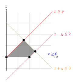
- $\max x+y$ ? Yellow line.
- $\max 2y+x$ ? Only at $x=1.5, y=1.5$ .

Why bother?

Optimization on Boolean functions: weighted model counting over $(\max,+)$ -semiring.

Naive formulation:

$\max \sum_{i=1}^n \alpha_i x_i + \beta_i(1-x_i)$
$\text{s.t}.~(x_1,\dots,x_n) \models f$

Relaxed formulation

$\max \sum_{i=1}^n \alpha_i x_i + \beta_i(1-x_i)$
$\text{s.t}.~(x_1,\dots,x_n) \in conv(f)$

We know that the optimal value is reached on an extreme point, hence at a model of $f$ .

Both version have the same optimal value.

The definition of $conv(f)$ involves $n+\#f$ variables.

Not better than going over every model of $f$ .

Extension Complexity

Challenge: find a succinct representation of $conv(f)$ .

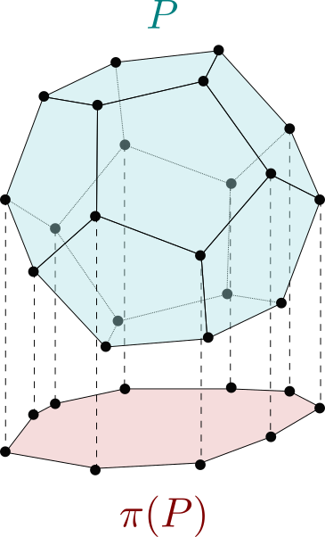
Extension complexity: write a polyhedron on dimension $n$ as the projection of a polyhedron on dimension $n+K$ . Smallest possible $K$ .

$conv(f)$ : we know how to do $K = \#f$ . Can we do better?
Extension complexity of $f$ !

Extension Complexity of OBDD

OBDD and paths

Complete OBDD: models = paths.

Path corresponds to

$e_1=e_3=e_7=1$ ,
$e_2=e_4=e_5=e_6=e_8=0$
$x=1, y=1, z=1$ .

Integer linear constraints describing paths:

$1 = e_1+e_2$	$x = e_1$
$e_1 = e_6+e_7$	$y = e_3+e_5$
$e_2 = e_5+e_6$	$z = e_7$
$e_2 = e_5+e_6$
$e_3+e_6=e_7$
$e_5+e_4=e_8$
$e_1 \in \{0,1\}, \dots, e_8 \in \{0,1\}$

Relaxing paths

Corresponds to point $x = 1/3, y=2/3, z=2/3$ , or convex combination:

$(1/3) \cdot (1,1,1)+ (1/3) \cdot (0,1,0) + (1/3) \cdot (0,0,1)$

Solutions to the relaxed program = flows

Integral solutions = models

Extreme points of flows are integral.

$\Rightarrow$ Projection of the linear program on $(x,y,z)$ is $conv(f)$ .

Relax previous program:

$1 = e_1+e_2$	$x = e_1$
$e_1 = e_6+e_7$	$y = e_3+e_5$
$e_2 = e_5+e_6$	$z = e_7$
$e_2 = e_5+e_6$
$e_3+e_6=e_7$
$e_5+e_4=e_8$
$e_1 \in$ [0,1], $\dots, e_8 \in$ [0,1]

Wrap up on OBDD

If $f(x_1,\dots,x_n)$ is computed by an OBDD of size $C$ having $m$ edges, $conv(f)$ can be describe with $n+m$ contraints (expressing, intuitively, a source-sink flow in the OBDD).

Application:

Maximize linear function over the models of $f$ in polynomial time (not really interesting).
Allows to translate $\tau \models f$ as a system of linear constraints in linear programs

Extension Complexity of DNNF

DNNF and Proof trees

Smooth DNNF: models = proof tree

Pick one edge for $\vee$ -gates
Both edges for $\wedge$ -gates
Until inputs reached: $x_1=0, x_2=1, x_3=1, x_4=1$

Linear program encoding of proof trees

One variable $e \in \{0,1\}$ per edge of the DNNF:

Encoding $\vee$ -gates:

one output edge is selected
exactly one input edge is selected

$f_1 + \dots + f_p = e_1 + \dots + e_k$

Encoding $\wedge$ -gates:

one output edge is selected
every input edge is selected

$f_1 + \dots + f_p = e_i$ for every $i \leq k$

Encoding the model:

$x = f_1 + \dots + f_p$

Linear program : relaxation

Relax $e \in \{0,1\}$ to $e \in [0,1]$ .

Bounded polyhedron, described with $O(n+m)$ constraints ( $m$ number of edges)
Integral points are exactly the proof trees hence the models of $f$
Are there non-integral extreme points?

We can show that the relaxed program is integral: every extreme point has integer coordinates.

It is an extended formulation of $conv(f)$ !

Applications

Binary Polynomial Optimization

$\max \sum_I \alpha_I \prod_{i\in I} x_i \qquad~~~ (x_1,\dots,x_n) \in \{0,1\}^n$

NP-hard but extensive research on finding tractable instances.
Optimization theory origin: explain tractability in terms of extended formulations.

Boolean function encoding:

$\bigwedge_{I} (y_I \Leftrightarrow \bigwedge_{i \in I} x_i)$

Compile to DNNF:
- Solve weighted $(\max,+)$ -counting with $\alpha_I$ as weight of $y_I$ and $0$ for other literals.
- Extract extended formulation!

MSO Optimization

Monadic Second Order Logic:
- First order variables
- Second order variables that are “subset of elements”.

$3COL(C_1, C_2, C_3) = \forall x. (x \in C_1 \vee x \in C_2 \vee x \in C_3) \wedge \bigwedge_{i=1}^3 \forall x \forall y (C_i(x) \wedge C_i(y) \Rightarrow \neg E(x,y))$

Graph G=(V,E)G = (V,E): G⊨3COL(V1,V2,V3)G \models 3COL(V_1,V_2,V_3) if V1,V2,V3⊆VV_1,V_2,V_3 \subseteq V is a 3-coloring of GG.
- One Boolean variable $X_{x,C_i} \in \{0,1\}$ encodes $x \in C_i$ .
- For a fixed graph $G$ , encode solutions as Boolean functions $f_G$ .
Courcelle Theorem: If $G$ has treewidth $k$ , $f$ is computed by a d-DNNF of size $w(k) \cdot |G|$ .
Corollary: $conv(f)$ has extended formulations of size $O(w(k) \cdot |G|)$ .

[1] Kolman, Petr, Martin Koutecký, and Hans Raj Tiwary. “Extension complexity, MSO logic, and treewidth.” Discrete Mathematics & Theoretical Computer Science 22.Discrete Algorithms (2020).

Conclusion

Take home message

DNNF can be used to construct extended formulations:
- Original motivation of the result
- “Linearize” convex but non-linear constraints
- Applications to BPO: $\max \sum_{I} \alpha_I \prod_{i \in I} x_i$ over $\{0,1\}^n$
- Applications to bounded treewidth MSO
Extended formulation of conv(f)conv(f) can be seen as a representation language for Boolean function:
- At least as succinct as DNNF
- Support conditioning, existential projection, linear optimization, enumeration (?)

A model counting question

FPRAS:

Number o fmodels of a DNNF [Meel, De Colnet].
Knapsack [Dyser]

What about extended formulations of $conv(f)$ ?

Futur work

Explore Extended Formulations as represensation languages :
- Mapping tractable queries and transformations
- How can we compile into them appart from building DNNF?
- Separation with DNNF?
- Lower bounds? Interesting connections with previous work.
Study “determinism” from a linear program perspective
- What kind of extended formulation do we get?
- Can we generalize them to support model counting?

Extension Complexity and the Convex Hull of Boolean Functions