Introduction

Problems & solutions

000000

000001

000010

000011

000100

000101

000110

000111

001000

001001

001010

001011

001100

001101

001110

001111

010000

010001

010010

010011

010100

010101

010110

010111

011000

011001

011010

011011

011100

011101

011110

011111

100000

100001

100010

100011

100100

100101

100110

100111

101000

101001

101010

101011

101100

101101

101110

101111

110000

110001

110010

110011

110100

110101

110110

110111

111000

111001

111010

111011

111100

111101

111110

111111

Is there a green box satisfying a set of “constraints”?

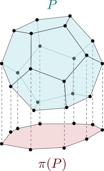
Understanding the set of solutions

000000

000001

000010

000011

000100

000101

000110

000111

001000

001001

001010

001011

001100

001101

001110

001111

010000

010001

010010

010011

010100

010101

010110

010111

011000

011001

011010

011011

011100

011101

011110

011111

100000

100001

100010

100011

100100

100101

100110

100111

101000

101001

101010

101011

101100

101101

101110

101111

110000

110001

110010

110011

110100

110101

110110

110111

111000

111001

111010

111011

111100

111101

111110

111111

Open every box? Works, but costly.

Open every green box? Still costly: full materialization.

Is there a middle ground between implicit and fully explicit?

Count the green boxes? Pick a green box uniformly at random. Find every green box. Find “the best” green box. Count the green boxes starting with 0

From implicit definition to ?

$b_1~~b_2~~b_3~~b_4~~b_5~~b_6$

$b_1~~b_2~~b_3$ $b_4~~b_5~~b_6$

List of constraints:

$\neg b_1 \vee \neg b_2 \vee b_3$
$\neg b_1 \vee \neg b_2 \vee b_3$
$b_1 \vee \neg b_2 \vee \neg b_3$
$b_1 \vee b_2 \vee b_3$

$\neg b_4 \vee \neg b_5 \vee \neg b_6$
$\neg b_4 \vee b_5 \vee b_6$
$b_4 \vee \neg b_5 \vee b_6$
$b_4 \vee b_5 \vee \neg b_6$

$(b_1~b_2~b_3)$ has an even number of $1$ .

$(b_4~b_5~b_6)$ has an odd number of $1$ .

Solutions are described by circuits using Cartesian products and (possibly disjoint) unions!

Here we can deduce that there are $4 \times 4 = 16$ solutions!

Circuits Zoo

DNNF

\{\cup,\times\}

-circuits

x	y
0	0
0	1
0	2
1	0
1	1
1	2

deterministic DNNF

\{\uplus,\times\}

-circuits

decision DNNF

\{\mathsf{dec},\times\}

-circuits

x₁	x₂	x₃
0	0	0
1	2	1
2	2	2
…

$\uplus$ allows for counting!

Knowledge Compilation Map

Visualize the properties of each circuit class:

Gates	Boolean Domain	Enum	Count	Condition	Complement
$\{\cup, \times\}$	DNNF	☑	❌	✅	❌
$\{\uplus, \times\}$	d-DNNF	✅	✅	✅	❌
$\{\mathsf{dec}, \times\}$	dec-DNNF	✅	✅	✅	❌
$\{\mathsf{dec}\}$	FBDD	✅	✅	✅	✅

The goal of knowledge compilation is to build, exploit and understand the limits of compact yet tractable representations of an implicitly defined set.

Selected Contributions

Building small representations

New algorithms inspired by model counting
with Bova, Mengel, Slivovsky
New canonical datastructure called TDD.
with Choi, Mengel, Muñoz, Van den Broecke
New analysis of exhaustive DPLL .
with Carmeli, Irwin, Salvati

Lower bounds and limits

Lower bounds and communication complexity
with Bova, Mengel, Slivovsky
Sharp lower bounds based on treewidth.
with Amarilli, Monet, Senellart

Finding new applications

Applications to certifying model counters.
with Lagniez, Marquis
Solving linear programs over databases.
Nicolas Crosetti’s thesis with Niehren, Ramon, Tison
Applications to direct access
Oliver Irwin’s thesis Salvati
Applications to optimization problems.
with Del Pia and Di Gregorio

Building Circuits

Constraints

Input: constraints $F \coloneq R(x_1, x_2) \wedge S(x_1, x_3) \wedge T(x_2, x_3)$ .

$F_2 \coloneq R(x_1, x_2) \wedge S(x_1, x_3) \wedge \neg T(x_2, x_3)$ .

Output: the set of assignments of variables satisfying every constraint

$R$	$x_1$	$x_2$
	0	0
	0	1
	2	1

$S$	$x_1$	$x_3$
	0	0
	0	2
	2	3

$T$	$x_2$	$x_3$
	0	2
	1	0
	1	2

$F$	$x_1$	$x_2$	$x_3$
	0	0	2
	0	1	0
	0	1	2

$F_2$	$x_1$	$x_2$	$x_3$
	0	0	0
	2	1	3

Boolean functions: CNF formula, ie, constraints of the form $x_1 \vee \neg x_2 \vee x_3$
Database: joining tables

Materialization can be costly. Can we avoid it by constructing circuits?

Building circuits Top Down

Branching algorithm known as exhaustive DPLL:

$F = (\neg x_4 \vee x_5) \wedge (\neg x_1 \vee x_2 \vee x_3) \wedge (\neg x_2 \vee \neg x_3) \wedge (x_1 \vee x_4 \vee x_5) \wedge (\neg x_1 \vee \neg x_4 \vee \neg x_5) \wedge (x_1 \vee x_2 \vee x_3)$

$(\neg x_4 \vee x_5) \wedge (\neg x_1 \vee x_2 \vee x_3) \wedge (\neg x_2 \vee \neg x_3) \wedge (x_1 \vee x_4 \vee x_5) \wedge (\neg x_1 \vee \neg x_4 \vee \neg x_5) \wedge (x_1 \vee x_2 \vee x_3)$ $(\neg x_4 \vee \neg x_5) \wedge (\neg x_4 \vee x_5) \wedge (x_2 \vee x_3) \wedge (\neg x_2 \vee \neg x_3)$ $(\neg x_4 \vee \neg x_5) \wedge (\neg x_4 \vee x_5)$ $(x_5) \wedge (\neg x_5)$ $()$ $(x_5) \wedge (\neg x_5)$ $()$ $(x_5) \wedge (\neg x_5)$ $(\neg x_4 \vee \neg x_5) \wedge (\neg x_4 \vee x_5)$ $(\neg x_4 \vee \neg x_5) \wedge (\neg x_4 \vee x_5)$ $(\neg x_4 \vee \neg x_5) \wedge (\neg x_4 \vee x_5)$ $\wedge (x_2 \vee x_3) \wedge (\neg x_2 \vee \neg x_3)$ $(x_2 \vee x_3) \wedge (\neg x_2 \vee \neg x_3)$ $(\neg x_4 \vee \neg x_5) \wedge (\neg x_4 \vee x_5) \wedge$ $(x_2 \vee x_3) \wedge (\neg x_2 \vee \neg x_3)$ $(\neg x_4 \vee x_5) \wedge (\neg x_1 \vee x_2 \vee x_3) \wedge (\neg x_2 \vee \neg x_3) \wedge$ $(x_1 \vee x_4 \vee x_5)$ $\wedge (\neg x_1 \vee \neg x_4 \vee \neg x_5) \wedge$ $(x_1 \vee x_2 \vee x_3)$ $(x_4 \vee x_5) \wedge (\neg x_4 \vee x_5) \wedge (x_2 \vee x_3) \wedge (\neg x_2 \vee \neg x_3)$ $(x_4 \vee x_5) \wedge (\neg x_4 \vee x_5)$ $\wedge (x_2 \vee x_3) \wedge (\neg x_2 \vee \neg x_3)$ $(x_2 \vee x_3) \wedge (\neg x_2 \vee \neg x_3)$ $(x_4 \vee x_5) \wedge (\neg x_4 \vee x_5) \wedge (x_2 \vee x_3) \wedge (\neg x_2 \vee \neg x_3)$ $(\neg x_4 \vee x_5) \wedge$ $(\neg x_1 \vee x_2 \vee x_3)$ $\wedge (\neg x_2 \vee \neg x_3) \wedge (x_1 \vee x_4 \vee x_5) \wedge$ $(\neg x_1 \vee \neg x_4 \vee \neg x_5)$ $\wedge (x_1 \vee x_2 \vee x_3)$

Exhaustive DPLL in practice

Used in practice by many knowledge compiler (d4, sharpSAT, sharpSAT-TD, Ganak etc.).

SAT solver calls to cut dead branches.
Use learnt clauses to find unit literals to propagate.
Heuristics for picking the next variable.

Exhaustive DPLL and Databases

Collaboration with Oliver Irwin during his thesis :

Exhaustive DPLL gives an efficient algorithm for computing database join queries with negations
Size of the circuit: depends on the order $\pi=(x_1,\dots,x_n)$ chosen on variables.
- Size bounds of the form $O(|\mathbb{D}|^{k})$ where $k = \iota(Q,\pi)$ .
- Circuits allow to recover the $i^{th}$ tuple wrt lexicographical order in time $O(\log |\mathbb{D}|)$ .
- Optimal complexity under reasonable complexity assumption.

In this case, the circuit behaves as a compressed table with efficient indexing.

Generalizes and unify previous results by Bringmann, Carmeli, Mengel.

Building circuits bottom-up

OBDD: $\{\mathsf{dec}\}$ -circuits with a total order on variables

OBDDs enjoy two properties:

Given OBDD $C_1, C_2$ , we can produce a new OBDD computing $C_1 \wedge C_2$ of size $\leq |C_1| \cdot |C_2|$ .
Given an OBDD $C$ , we can produce an equivalent minimal canonical OBDD.

pi = order(F) # choose a "good" order
d = OBDD(1, pi)
for c in F:
    d2 = OBDD(c, pi) # create an OBDD for the clause
    d.apply(d2)  # apply the clause 
    d.minimize() # minimize
return d

Generalizing OBDD

OBDD are not succinct enough: path structure misses a lot of decompositions.

Tree Decision Diagrams (TDD): a new treelike generalization of OBDD.
Chapter 2 of the manuscript; accepted at SAT26 with YooJung Choi, Stefan Mengel, Martín Muñoz, Guy Van den Broecke

Determinism

TDD must respect the following determinism condition: a pair of siblings can be the input of at most one parent node.

Wonderful TDDs

TDD can be minimized into a canonical form by iteratively merging twin nodes.
TDD support apply.

T = vtree(F) 
d = TDD(1, T)
for c in F:
    d2 = TDD(c, T) 
    d.apply(d2) 
    d.minimize() 
return d

Efficient bottom-up compilation
More succinct than OBDD, simpler than SDD
Can efficiently represent bounded treewidth instances
- Proof by upper bounding the canonical TDD size.
- Gives insight on how to choose the vtree
TiDiDi compiler: promising experimental results.

Certifying #SAT Solvers

Trusting the tools

CNF Formula

$x \vee \neg y \vee z$
$x \vee y \vee \neg w$
…

SAT
because $x=0,y=1...$ is a model

UNSAT
Proof deriving a contradiction

Proving that $F$ has 42 models:

List 42 models
Prove that they are the only ones.
Does not scale

Give a succinct representation $C$ of all models
Prove that $C$ represents exactly the models of $F$
Closer to how #SAT solvers work.

Getting a succinct representation

Many #SAT solvers build (implicitly) a $\{\mathsf{dec},\times\}$ -circuit by applying Exhaustive DPLL.

CNF Formula

$(\neg x_4 \vee x_5)$

$(\neg x_1 \vee x_2 \vee x_3)$

$(\neg x_2 \vee \neg x_3)$

$(x_1 \vee x_4 \vee x_5)$

$(\neg x_1 \vee \neg x_4 \vee \neg x_5)$

$(x_1 \vee x_2 \vee x_3)$

8 models

Certifying the model count boils down to certifying that the circuit has the same models as the CNF.

Hardness of proving equivalence

Given a CNF formula $F$ and the circuit $C$ produced by a #SAT-solver:

Checking $C \Rightarrow F$ is easy (PTIME) by checking $\neg F \Rightarrow \neg C$ .
Checking $F \Rightarrow C$ is hard (coNP-hard): UNSAT formulas are represented by $\bot$ .

We need a device for making $F \Rightarrow C$ easy to check.

Annotating $\bot$ -gates

We want to check $F \Rightarrow C$ or equivalently $\neg C \Rightarrow \neg F$ : explain $\bot$ -gates!

$c_0 := \neg x \vee \neg y_1 \vee y_2$
$c_1 := \neg x \vee y_1 \vee \neg y_2$
$c_2 := \neg x \vee \neg z_1 \vee z_2$
$c_3 := \neg x \vee z_1 \vee \neg z_2$
$c_4 := \neg x \vee \neg z_2 \vee z_3$
$c_5 := \neg x \vee \neg z_3 \vee z_4$
$c_6 := x \vee y_1$

kcps proof system! [SAT, 2019]

Syntactic Entailment

Circuits produced by #SAT-solvers on input $F$ have a specific form:

Caching is syntactic, based on equivalence.
Each gate maps to a recursive call / subformula of $F$ .
Can be checked in ptime.

We use this idea to output certify d4 [C., Lagniez, Marquis, AAAI 2021].

$F = (x \vee y_1) \wedge (\neg x \vee y_2) \wedge (y_1 \vee \neg y_2) \wedge (\neg y_1 \vee y_2)$ .

$F[x] = y_2 \wedge (y_1 \vee \neg y_2) \wedge (\neg y_1 \vee y_2) \neq y_1 \wedge (y_1 \vee \neg y_2) \wedge (\neg y_1 \vee y_2) = F[\neg x]$

$F[x,y_1] = F[\neg x, y_1]$

Proof System Landscape

Many proof systems for #SAT boils down to certifying $F \Rightarrow C$ .
Insight of Chapter 3 and [Beyersdorff, Hoffmann, Kasche 2026]: MICE is a particular form of syntactic equivalence

CLIP: [Chede, Chew, Shukla 2024]

CPOG: [Bryant, Nawrocki, Avigad, Heule 2023]

MICE: [Fichte, Hecher, Roland 2022]

MICE (Semantic/Reference): [Beyersdorff, Hoffmann, Kasche 2026]

$T_{sparse}/T_{dense}$ : [Beyersdorff, Giesen, Goral, Hoffmann, Kasche, Staudt 2026]

Convex Optimization

Optimizing Boolean function

Optimization on Boolean functions:

Naive formulation:

$\max \sum_{i=1}^n \alpha_i x_i + \beta_i(1-x_i)$
$\text{s.t}.~(x_1,\dots,x_n) \models f$

Relaxed formulation

$\max \sum_{i=1}^n \alpha_i x_i + \beta_i(1-x_i)$
$\text{s.t}.~(x_1,\dots,x_n) \in conv(f)$

$f$	$x$	$y$
$\vec{v}_0$	0	0
$\vec{v}_1$	1	0
$\vec{v}_2$	0	1

Both problem have the same optimal value. Can we describe $conv(f)$ with a small number of linear constraints?

OBDD

Complete OBDD: models = paths.

$x=1, y=1, z=1$ .
$e_1=e_3=e_7=1$ ,
$e_2=e_4=e_5=e_6=e_8=0$

$x=1/3$ $y=z=2/3$
$e_1=e_3=e_5=e_6=e_8=1/3$ $e_2=e_7=2/3$
$e_4=0$

Integer linear constraints describing paths:

$1 = e_1+e_2$	$x = e_1$
$e_1 = e_6+e_7$	$y = e_3+e_5$
$e_2 = e_5+e_6$	$z = e_7$
$e_2 = e_5+e_6$
$e_3+e_6=e_7$
$e_5+e_4=e_8$
$e_1 \in \{0,1\}, \dots, e_8 \in \{0,1\}$ $e_1 \in [0,1], \dots, e_8 \in [0,1]$

Projection of the linear program on $(x,y,z)$ is $conv(f)$ .

Extension complexity of OBDD

If $f(x_1,\dots,x_n)$ is computed by an OBDD having $m$ edges, $conv(f)$ can be describe with $O(n+m)$ linear contraints.

Such system is called an extended formulation of $conv(f)$ .

Extension Complexity of $\{\cup,\times\}$ -circuits

Write linear program encoding proof trees
Relax in $[0,1]$ .
Show that the linear program is integral (***)

If $f(x_1,\dots,x_n)$ is computed by an $\{\cup,\times\}$ -circuit having $m$ edges, $conv(f)$ can be describe with $O(n+m)$ linear contraints.

Applications

Binary Polynomial Optimization

$\max \sum_I \alpha_I \prod_{i\in I} x_i \qquad~~~ (x_1,\dots,x_n) \in \{0,1\}^n$

Compile to $\{\cup,\times\}$ -circuit.
Extract extended formulation!
PoC with d4.

Collaboration with Alberto Del Pia and Silvia Di Gregorio.

CQ and Linear programs

Linear programs whose variables are the answers of a Conjunctive Query.
Compile into $\{\times,\uplus\}$ -circuits.
Solve smaller linear program!

Nicolas Crosetti’s thesis (collaboration with Joachim Niehren and Jan Ramon).

MSO Optimization

Monadic Second Order Logic.
Known representation in $\{\uplus,\times\}$ -circuits
Give extended formulations for such problems (e.g., vertex cover)

Recover results from “Extension complexity, MSO logic, and treewidth.” by Kolman, Koutecký and Tiwary.

Algorithmic Applications of Knowledge Compilation

Introduction

Problems & solutions

Understanding the set of solutions

From implicit definition to ?

Circuits Zoo

Knowledge Compilation Map